p1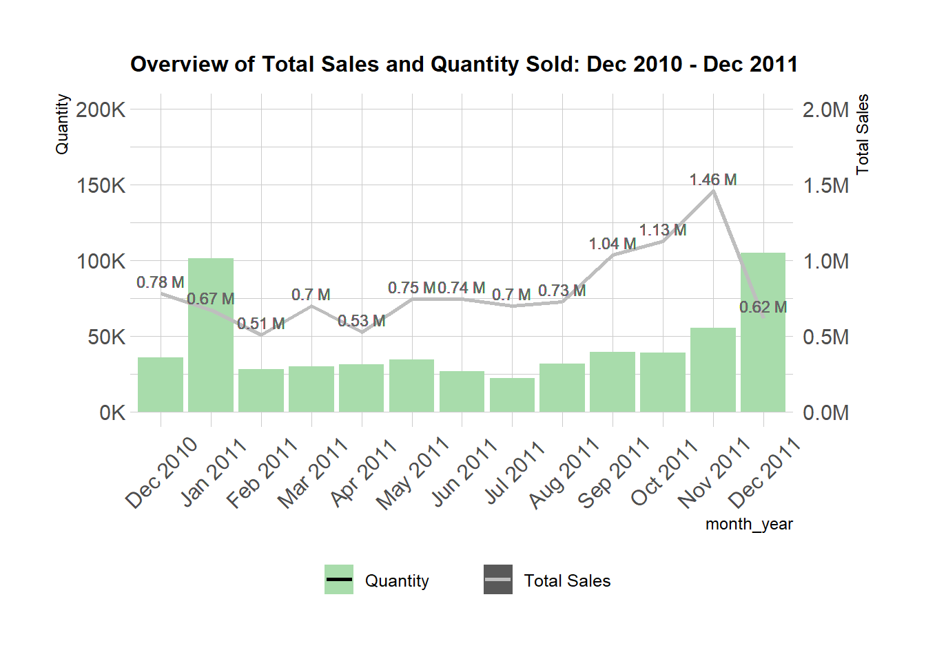
This analysis utilizes open-sourced data from kaggle. Online Retail Dataset The dataset contains online retail transaction records from a UK-based online retail business. A Business health analysis was conducted to assess the company’s long-term sustainability.
p1
Graph above shows a stable stream of income from month Dec 2010 to Dec 2011. Business revenue peaked in November 2011 with 1.46 million and reach the lowest point in December 2011 at 0.62 million. Total monthly Quantity sold remains above 30k units regardless product categories.
p2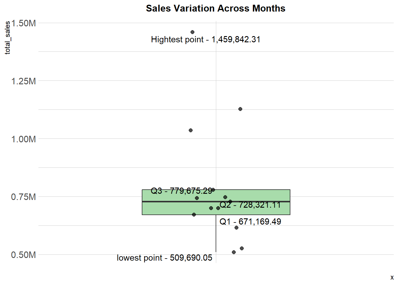
Monthly sales distribution shows center 50% of monthly revenue values fall within 0.67 million to 0.78 million. The spread from median (Q2) to lowest point is 0.27 million while the spread from Q2 to highest point 0.73 million. This indicates business faces relative low downside risk, as the fluctuations below Q2 are smaller.In contrast, the upside potential is significant, given the larger spread above Q2. Business should investigate the underlying factors that contributed to months where total sales exceeded Q3. If these success drivers are replicable, they should be integrated into a long-term business strategy.
#data calculation from sales.qmd
read_file("total_quantity_sold_and_stock_return_by_category.rds") %>%
  group_by(category, type) %>%
  mutate(
    total_quantity = sum(total_quantity)
  ) %>%
  distinct() %>%
   barchart_ggv2(.,category, total_quantity, fill = type, stack = F)+
  coord_flip()+
  labs(
    title = "Overview: Total Quantity Sold and Sales Returns by Category"
  )+
  theme_function(title_size = 12)+
  scale_y_continuous_function(0,2800000,m)+
  geom_text_function(repel = F, stack = F, vjust = 0.5, hjust = -0.25, label = comma(total_quantity))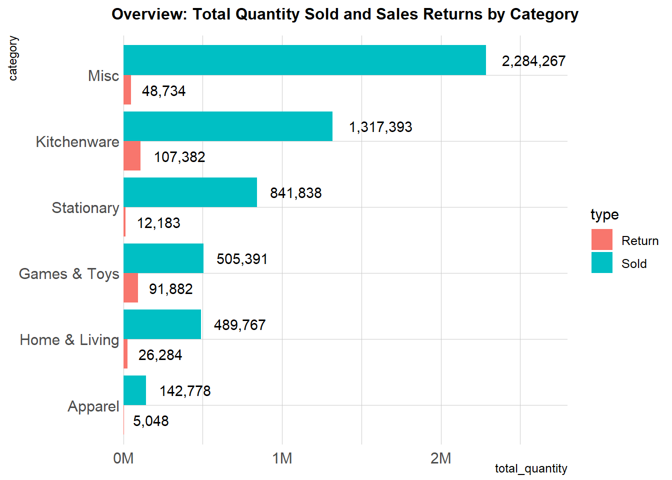
The graph above provide an overview of the contribution of product categories to business’s revenue and corresponding sales returns. Particular attention should be paid to the quantity of sales returns, as the returned amounts are signicant - even though most category have returns below 10 percents of quantity sold, except for Games and Toys.
To visualize the potential loss, sales return have been monetized. The calculation base on:
average Sale Price per unit * Quantity of Sale Returns
(Note: Cost of goods sold is unavailable in the dataset.)
Result as per below:
#calculation from sales.qmd
read_file("losses_from_return_table.rds") %>%
    kbl(caption = "Losses Incurred from Sales Returns") %>%
kable_styling()| category | total_lost |
|---|---|
| Apparel | 9,566.25 |
| Stationary | 15,523.56 |
| Home & Living | 54,134.16 |
| Kitchenware | 161,520.50 |
| Games & Toys | 187,197.46 |
| Misc | 236,307.16 |
| Accumated losses ($) | 664,249.09 |
Table above shows losses incurred in each category. Result indicates total potential revenue from Dec 2010 to Dec 2011 is 0.66 million, which is similar to busines’s average monthly revenue. It is hoped that this demontration will capture the attention of business owner and prompt action to investigate the underlying causes.
Data uncovers hints of structural weaknesses in database, casting doubt on the quality and reliability of data analysis. Those hints include:
StockCode, Quantity and UnitPrice are jointly used to record business expenses (ie, commission, postage, bank chages), sales and sales return.StockCode is assigned to business expenses. (ie, commission, postage, bank charges)Descriptionare inconsistent.read_file("Total Wastage.rds") %>%
barchart_ggv2(
data = .,
x_col = category,
y_col = total_wastage,
stack = F,
fill_color = category
)+
coord_flip()+
labs(
title = "Overview: Total Write Off Goods in Units (Dec 2010 to Dec 2011)"
)+
theme_function(
title_size = 12,
legend = F,
margin_plot = margin(t=20, b=20, r=20,l=10)
)+
geom_text_function(repel = F, hjust = -0.5,
label = paste0(
comma(total_wastage, accuracy = 1),
" units")
)+
scale_y_continuous_function(0, 100000, suffix = K)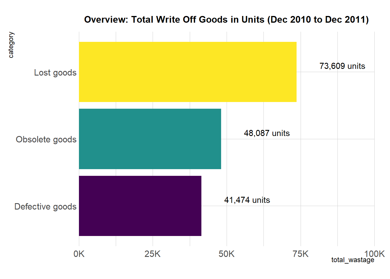
The graph above shows 163k units of goods in total were write off from December 2010 to December 2011. The business should take note, as the number of write offs exceeds than the highest recorded sales within the time frame.
Distribution of write offs to months as per below:
read_file("lost_good_per_month.rds") %>%
  linechart_gg(.,month_year, total)+
  labs(
    title = "Lost Goods by Month"
  )+
  scale_y_continuous_function(
    start_range = 0,
    end_range = 17000,
    suffix = K
  )+
  theme_function(
    x_label_position = element_text(angle = 45, vjust = 0.5),
    margin_y_title = margin(r=10),
    margin_x_title = margin(t=10)
  )+
  geom_text_function(
    repel = T,
    label = total,
    vjust = -0.8
  )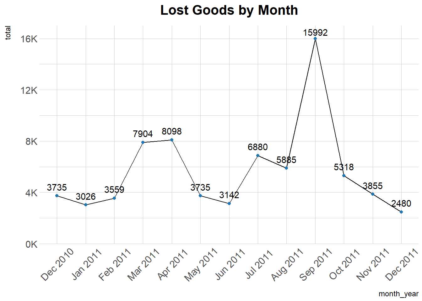
As illustrated in the graph above, loss of goods happened across all months. The number of losses ranging from as low as 2480 units to as high as 15,992 units. The business should conduct a thorough investigation and strengthen the existing inventory management system to prevent further losses.
read_file("obsolete_good.rds") %>%
  linechart_gg(.,month_year, total)+
  scale_y_continuous_function(
    start_range = 0,
    end_range = 30000,
    suffix = K
  )+
  labs(
    title = "Obsolete Goods by Month"
  )+
  theme_function(
    x_label_position = element_text(angle = 45, vjust = 0.5),
    margin_y_title = margin(r=10),
    margin_x_title = margin(t=10)
  )+
  geom_text_function(
    repel = T,
    label = total,
    vjust = -0.8
  )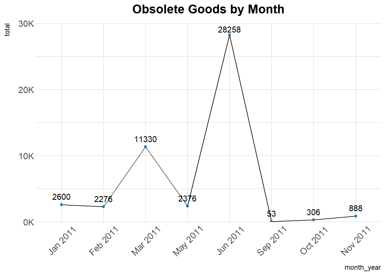
Graph above shows that goods were discarded across all months. The number of discards raised concerns whether appropriate control were taken place before such actions were taken.
read_file("defective_goods_by_month.rds") %>%
  linechart_gg(.,month_year, total)+
  scale_y_continuous_function(
    start_range = 0,
    end_range = 30000,
    suffix = K
  )+
  labs(
    title = "Defective Goods by month"
  )+
  theme_function(
    x_label_position = element_text(angle = 45, vjust = 0.5),
    margin_y_title = margin(r=10),
    margin_x_title = margin(t=10)
  )+
  geom_text_function(
    label = total,
    vjust = -0.8
  )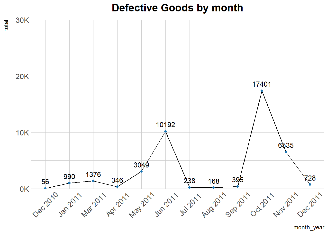
The graph above shows significant number of defective goods across all months. An investigation should be conducted to uncover the underlying causes and establish preventive procedures to minimize future losses.
The write off amount raises concerns on the effectiveness of inventory management system. The business to revise and consider improvement in areas, such as:
Policy should mandate management’s consent before write off action. Obsolete goods should cross checked by 2 parties. Photo of obsolete goods and management’s consent should be documented for audit purpose.
Policy should mandate monthly general cleaning, and prompt corrective actions must be taken if any signs of dampness are identified.
Policy should mandate a monthly product demand analysis to review the average demand of each product and establish or adjust the reorder point, in order to prevent overstocking of specific items.
Sample of calculation as per below:
#Reorder_point = (average daily demand * lead time) + Safety Stock
#safety_stock = Z * daily_demand_sd * sqrt(lead_time_days)
#max_stock_level = monthly_demand + safety_stock

#considering a postage delay of 1 month. Set buffer period of 5 days
#lead time day = 5 days
#daily average usage
#stock able to cover 95% of the time: z score = 1.65

read_file("reorder_level_per_stockcode.rds") %>%
  select(StockCode,average_sold_per_month, reorder_point, max_stock_level) %>%
  mutate(
    average_sold_per_month = round(average_sold_per_month,0)
  ) %>%
  distinct() %>%
result_displayv2(.,5,"")Policy should mandate management to periodically review the average demand for each product and discontinue underperforming items. Below is a list of products with a monthly demand of fewer than 5 units.
#considering some of the Stockcode has quantity sold less than 10 per month.
#it should be filter out to consider whether to drop the product
#Product that sold less than 5 units per month as per below

read_file("reorder_level_per_stockcode.rds") %>%
  filter(average_sold_per_month <= 5) %>%
  mutate(
    average_sold_per_month = round(average_sold_per_month,0)
  ) %>%
  select(StockCode, average_sold_per_month) %>%
  distinct() %>%
result_displayv2(.,5,"")While the business is currently performing well in terms of sales, it is essential to take appropriate measures to address the issues highlighted to support long-term sustainability.